Google TabFM — Tabular Foundation Models (zero-shot forecasting)

Last reviewed: 19 September 2026

Édition française : Google TabFM — Modèles de fondation tabulaires (prévision zéro-shot)

You have 84 rows of data — not 84 million. Can a tabular foundation model still predict, with no training and no tuning? This article explains how these models work, what they change compared with a classic data-science project, and tests them on a real case in Senegal: photovoltaic production against the electricity consumption of a house in Badoudou, near Sokone.

What you will understand

What a tabular foundation model is and why "tabular" means "spreadsheet": rows, columns, a target to predict.
The difference between learning by training (classic project) and learning in context (foundation model), illustrated diagram by diagram.
How TabFM from Google Research is built: attention by columns, compression of the rows, in-context learning Transformer.
How these models behave on a real small Senegalese dataset of solar production, against XGBoost/Random Forest/a linear regression.
When a foundation model is the right tool, and when it is not.

No prerequisite beyond secondary school: every notion is explained where it appears.

1. The problem: predicting well costs time, especially when data is scarce

A classic machine-learning project always follows the same path: you clean the data, you build useful variables, you choose a model, you tune its hyperparameters, you train it, you evaluate — and you start again. That work exists because the model starts from zero: it knows nothing about the world before seeing your data.

Direct consequence: the scarcer your data, the harder it is for the model to learn, and the more it risks learning your few rows "by heart" (overfitting). On 84 rows, a boosted decision tree can show 99% in training and be badly wrong on new data.

Foundation models turn the approach upside down: they have already learned how to learn, on hundreds of millions of synthetic tables, before meeting you.

2. The idea: a model that has seen millions of tables before yours

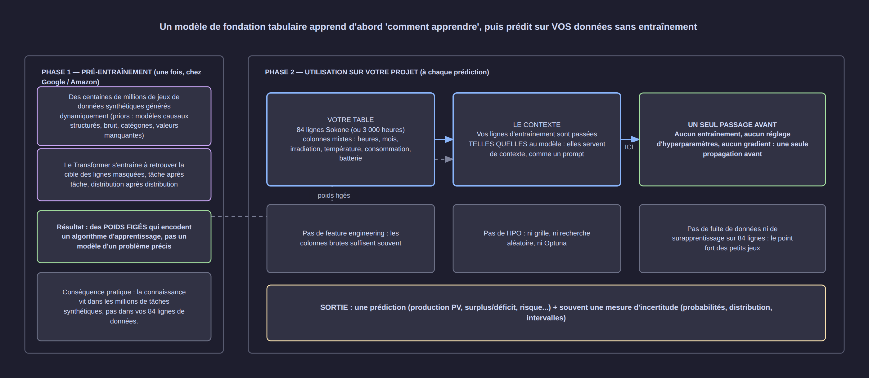
The principle comes in three steps:

Generate synthetic tasks. Millions of small "problems" are manufactured: random tables, with plausible causal structures (one variable influences another, some values are missing, some columns are categorical).
Train a Transformer to solve them. At each step, the model receives a table in which one column is masked and must reconstruct it. It is not trained on one problem: it is trained on the family of all problems.
Use the model on your data, with no training. Your training rows are passed to it as context, and it predicts the test rows in a single forward pass.

This last step is what is called in-context learning (in-context learning, ICL), by analogy with a language model that is given a few examples in the prompt rather than being retrained.

3. Classic project versus foundation model: what really changes

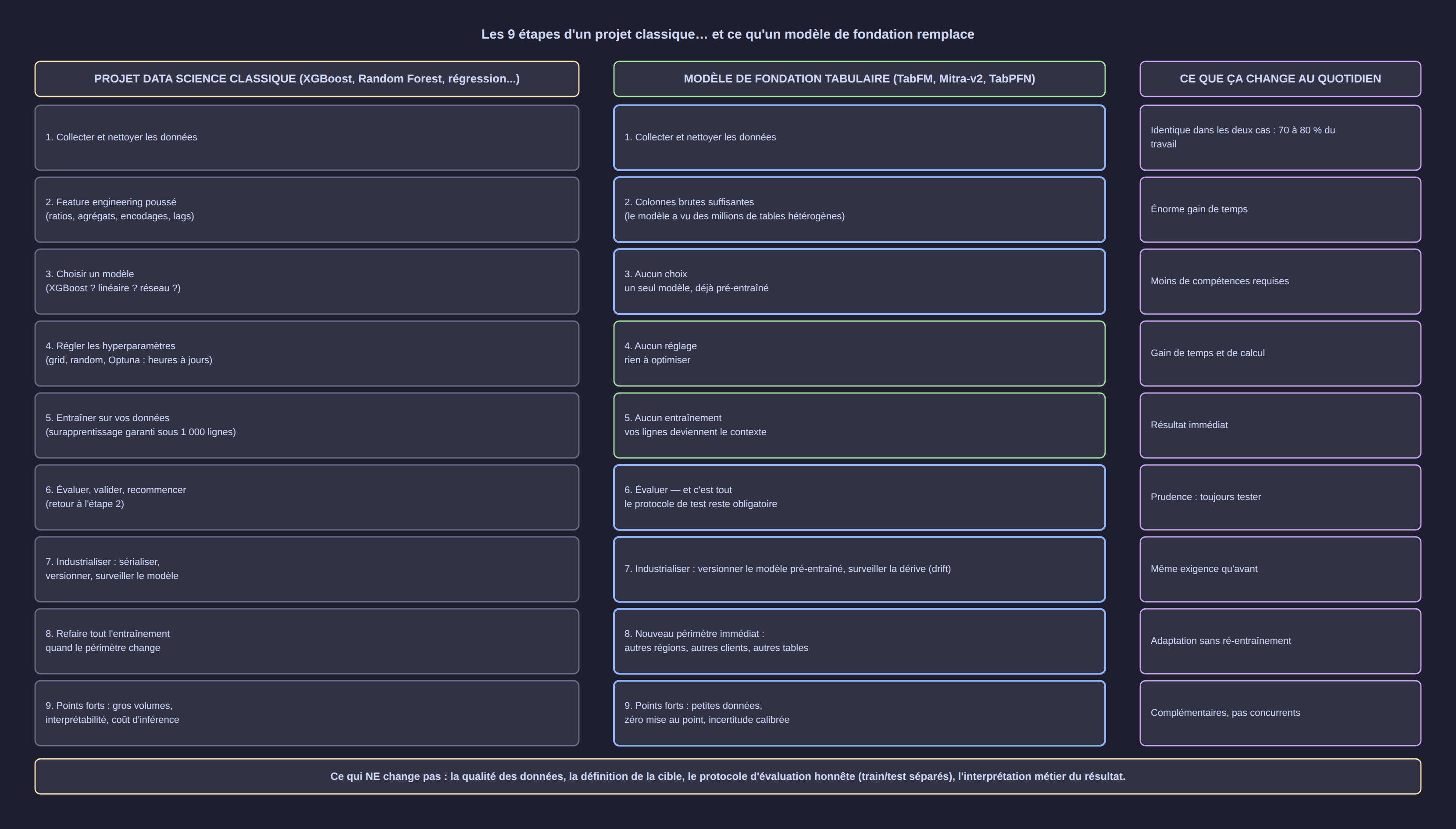
Step of a classic project	With a foundation model
Data cleaning	Identical — 70 to 80% of the work in both cases
Heavy feature engineering (ratios, aggregates, encodings, lags)	The raw columns are often enough
Model choice (XGBoost? linear? network?)	No choice: a single pre-trained model
Hyperparameter tuning (grid, random search, Optuna)	No tuning
Training on your data	No training: your rows become the context
Evaluation	Evaluation — the test protocol remains mandatory
Industrialisation (serialisation, versioning, drift)	Same requirement: version the pre-trained model, monitor drift
Full rework when the scope changes	New scope immediately: other regions, other clients, other tables

What does not change: data quality, the definition of the target, the train/test split, and the business interpretation of the result. A foundation model replaces neither the rigour nor the question asked; it replaces the tuning steps.

4. TabFM: how Google Research built it

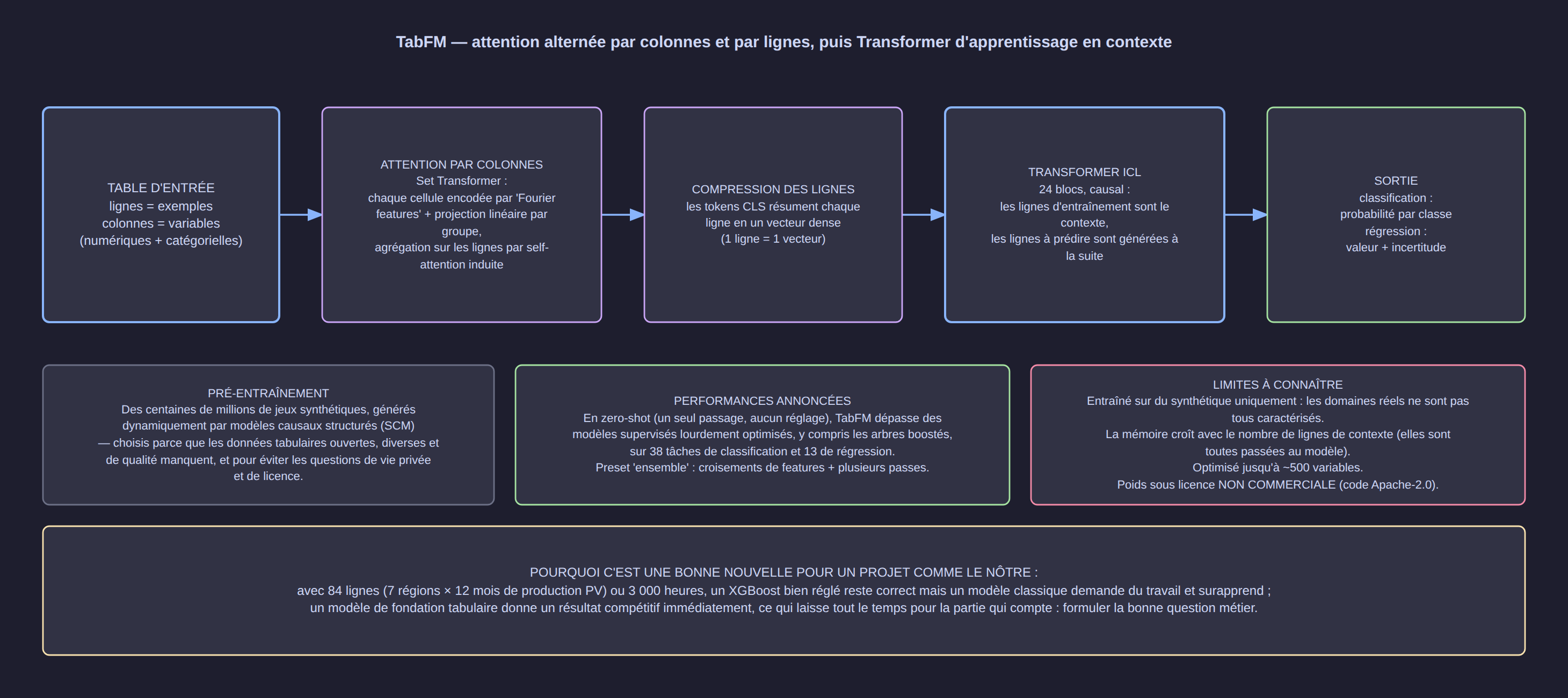
TabFM (Tabular Foundation Model, version 1.0.0, released in 2026) is a "zero-shot" tabular foundation model: it predicts the target of rows never seen before in a single pass.

Its architecture alternates two directions of attention:

Attention by columns. Each cell is encoded (Fourier features + linear projection per column group), then the columns aggregate the information across the rows through induced self-attention — the spirit of a Set Transformer. This is where the model learns the relationships between variables.
Row compression. CLS tokens summarise each row into a dense vector: a row becomes a point in a representation space.
In-context learning Transformer. 24 causal blocks process these row vectors: the training rows form the context, the rows to predict come "next".

TabFM was pre-trained on hundreds of millions of synthetic datasets generated dynamically from structured causal models (structural causal models). The choice of synthetic data is accepted by the authors: open, diverse and high-quality tables are missing, and real industrial data raises privacy and licensing questions.

According to the model card, in zero-shot mode (a single pass, no tuning), TabFM beats heavily optimised supervised models — boosted trees included — on 38 classification tasks and 13 regression tasks.

[!NOTE] Licence to check before any commercial use. The TabFM code is published under the Apache-2.0 licence, but the pre-trained weights are distributed under a "non-commercial" licence (tabfm-non-commercial-v1.0). For production use, you need either an authorisation or another model (TabPFN, Mitra-v2, or a classic model).

5. Learning in context, or changing the weights?

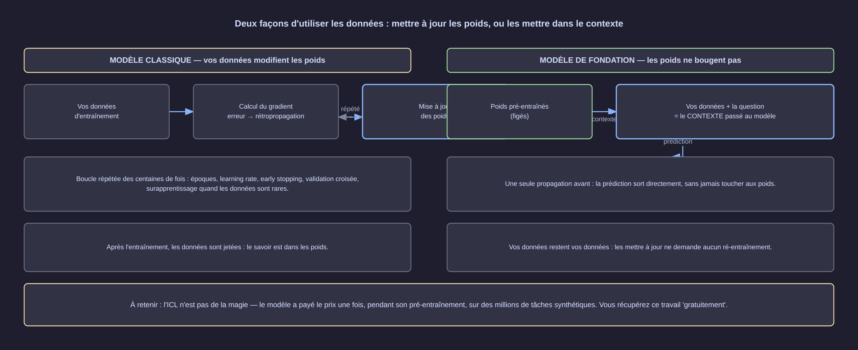
This is the most useful distinction to remember:

Classic model: your data is used to compute a gradient, which modifies the model's weights. You repeat that for whole epochs. At the end, the data is thrown away: the knowledge lives in the weights.
Foundation model: the weights stay frozen. Your data travels with the query, as a context. Changing dataset requires no retraining.

In practice, this means that a forecast for a new region, a new client or a new year takes a few seconds, not a night of computation.

6. The use case: a house in Badoudou (Sokone), PV production against consumption

6.1 The question asked

A house of 80 m², six people, near Sokone: what panel power and what battery capacity are needed for solar production to cover consumption, and can a foundation model help to forecast it?

6.2 The data: real first, synthetic only where necessary

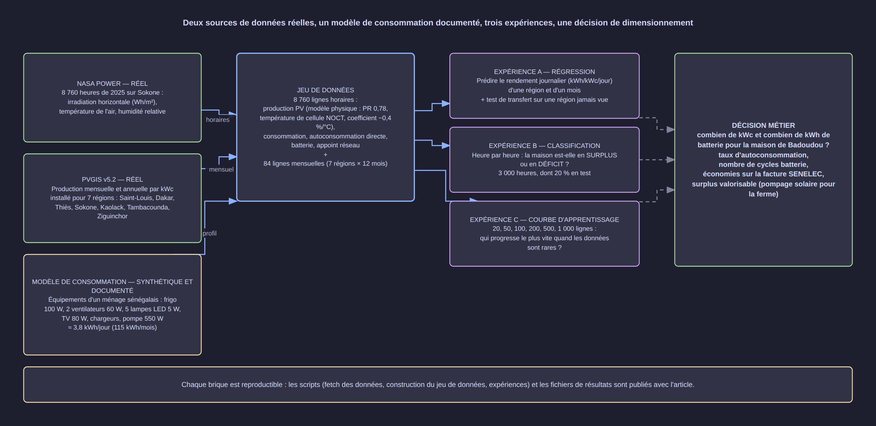
Source	Nature	Content
NASA POWER (public API)	Real	8,760 hours of the year 2025 at Sokone (13.8767° N, −16.3597° W): horizontal irradiation, air temperature, relative humidity
PVGIS v5.2 (European Commission)	Real	Monthly and annual photovoltaic production per kWp for 7 regions: Saint-Louis, Dakar, Thiès, Sokone, Kaolack, Tambacounda, Ziguinchor
Appliance model	Synthetic, documented	Consumption of a Senegalese household: 100 W refrigerator, two 60 W fans, five 5 W LED lamps, 80 W television set, phone chargers, 550 W pump

The consumption profile is an appliance model, not a measurement: each appliance has a known power rating, a duration of use and a seasonality (fans driven by temperature, longer lighting in the rainy season, pump in the dry season). Result: ≈ 3.8 kWh per day (115 kWh per month), consistent with an equipped rural household.

Photovoltaic production is calculated with a physical model, not invented: rated power × (irradiation / 1,000) × performance ratio (0.78), with thermal de-rating (−0.4%/°C, cell temperature estimated by the NOCT model at 45 °C).

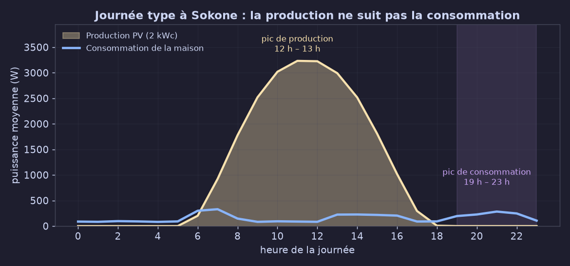
The figure above is the heart of the problem: production peaks at noon, consumption at 8 p.m. Everything that follows — battery, surplus, sizing — flows from this mismatch.

6.3 The experiment protocol — the part that makes the result credible

Three experiments, always with the same train/test split for all models:

Experiment A — regression. Predict the daily yield (kWh/kWp/day) of a region and a month: 84 rows (7 regions × 12 months). Protocol 1: random 85/15 split. Protocol 2: leave a whole region out of training and predict it — the real test of generalisation.
Experiment B — classification. Hour by hour, is the house in surplus (production

consumption) or in deficit? 1,500 hours sampled out of 8,760, 33% in the test set.
Experiment C — learning curve. 20, 50, 100, 200, 500 then 1,000 training rows: which one progresses fastest when data is scarce?

Models compared: mean/majority class (naive baseline), linear regression, Random Forest, HistGradientBoosting (boosted trees), and TabPFN v2 in zero-shot mode — the reference tabular foundation model that runs locally, from the same family of ideas as TabFM (in-context learning, no training on the user's data).

[!NOTE] Why TabPFN and not TabFM in the experiment? TabPFN v2 runs locally on CPU with public weights, which makes the experiment reproducible by anyone. TabFM's weights are under a non-commercial licence, and recent versions of TabPFN require licence acceptance and an API key. Version used: tabpfn 2.1.3. The conclusions concern the family of models (in-context learning), not a vendor.

6.4 Results

a) Random split (85% training / 15% test)

First level of difficulty: the rows are shuffled, each model sees a little of every region and must predict the 13 remaining rows.

Model	MAE (kWh/kWp/day)	RMSE	R²	Training time
Naive mean (baseline)	0.150	0.243	−0.01	—
Linear regression	0.126	0.159	0.56	0.01 s
HistGradientBoosting	0.124	0.151	0.61	0.06 s
Random Forest	0.067	0.093	0.85	0.23 s
TabPFN v2 zero-shot	0.025	0.030	0.98	0.43 s

With 71 training rows, the zero-shot foundation model obtains R² = 0.98 and an error of 0.025 kWh/kWp/day, i.e. 0.5% of the average daily production — with no tuning, in 0.4 second, whereas the boosted tree peaks at R² = 0.61. Note also the "naive mean" row: its R² is negative, which means it does worse than predicting the mean — that is the baseline every model must beat.

b) Predicting a region never seen before — 84 rows in total

The hardest test: one whole region is removed from training (12 rows) and the model is asked to predict its production. No model has ever seen that region.

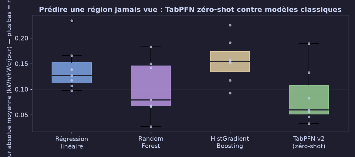
Held-out region	Linear regression (MAE)	Random Forest (MAE)	HistGradientBoosting (MAE)	TabPFN v2 zero-shot (MAE)
Dakar	0.166	0.183	0.192	0.133
Kaolack	0.127	0.068	0.093	0.046
Saint-Louis	0.118	0.150	0.154	0.190
Sokone	0.098	0.027	0.151	0.033
Tambacounda	0.234	0.079	0.118	0.059
Thiès	0.139	0.066	0.157	0.083
Ziguinchor	0.107	0.142	0.226	0.056
Mean	0.141	0.102	0.156	0.086

The unit is the kWh per kWp and per day. The average consumption of the dataset being 4.7 kWh/kWp/day, an error of 0.086 corresponds to about 1.8% relative error.

Put plainly:

Zero-shot TabPFN obtains the best average error (0.086) with no tuning at all, ahead of a hand-tuned Random Forest (0.102) and a boosted tree (0.156). Its average R² is 0.93.
Essential nuance: it loses on Saint-Louis (0.190 against 0.150 for the Random Forest) — the most productive region, the one it must extrapolate furthest from what it has seen. A foundation model is not magic: it is excellent at interpolation, more fragile at the extremes.
Linear regression is not ridiculous (0.141). It is the reminder that a simple baseline must always appear in the comparison: without it, you do not know whether the sophisticated model brings anything at all.

c) Predicting hour by hour: surplus or deficit?

The operational question — "at this hour, does the house produce more than it consumes?" — over 1,500 hours sampled across the year, one third kept for the test set (500 hours).

Model	Accuracy	F1 ("surplus" class)	AUC	Training time	Prediction time
Majority class (naive baseline)	55.6%	0.000	—	—	—
Logistic regression	99.39%	0.993	0.9998	0.01 s	< 0.01 s
Random Forest	99.60%	0.996	0.9999	0.36 s	0.02 s
HistGradientBoosting	99.80%	0.998	1.0000	0.11 s	0.01 s
TabPFN v2 zero-shot	100.00%	1.000	1.0000	0.16 s	472 s

What this table teaches — and it matters more than the ranking: when the target is almost deterministic (surplus is defined by production > consumption, and both are nearly known in the input variables), every serious model is excellent. The foundation model reaches 100% — but it takes 472 seconds to predict 500 rows on a CPU, against 0.01 second for a logistic regression that reaches 99.4%.

[!IMPORTANT] The right question is not "which model wins?" but "which model wins enough, at what cost?" A foundation model is precious when your data is scarce and the problem is hard; it is superfluous when a straight line already separates the classes. Here, the difference between 99.4% and 100% is probably not worth an inference time multiplied by 40,000.

d) How many rows do you really need?

This is the most instructive of the three experiments: the same models are trained with 20, 50, 100, 200, 500 then 1,000 rows, and accuracy is measured on the same test set.

Training rows	Random Forest	HistGradientBoosting	TabPFN v2 zero-shot
20	95.96%	55.56%	97.17%
50	95.56%	94.34%	98.79%
100	96.36%	99.39%	99.80%
200	98.79%	99.39%	99.80%
500	98.99%	99.60%	100.00%
1,000	99.60%	99.80%	100.00%

Reading: from 20 rows, the zero-shot foundation model is already at 97.2% — whereas the boosted tree is at 55.6% (it cannot learn with so little data) and the Random Forest needs 200 rows to reach a comparable level. This is exactly the operating regime of small projects: one field, one house, one client, one sensor. The foundation model is not only "as good": it is usable much earlier.

6.5 What the model really has to predict: sizing

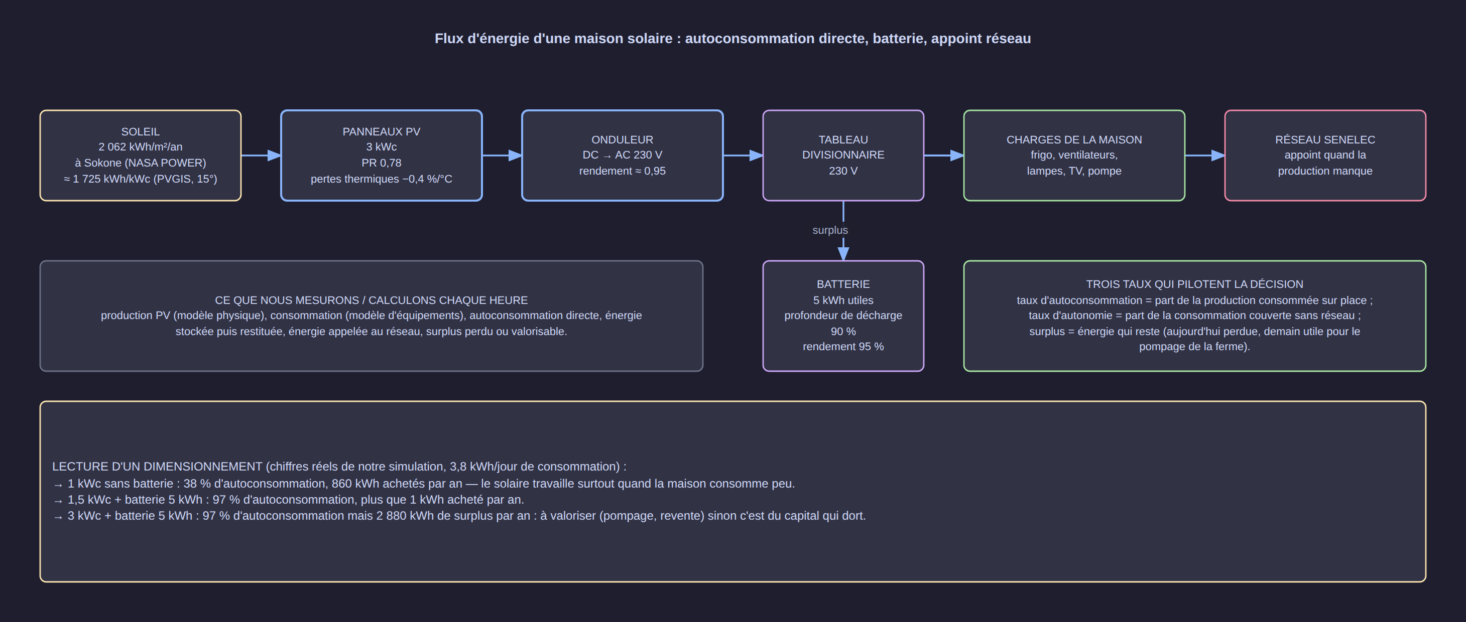
Once production and consumption are modelled hour by hour, the sizing question becomes a simple energy balance.

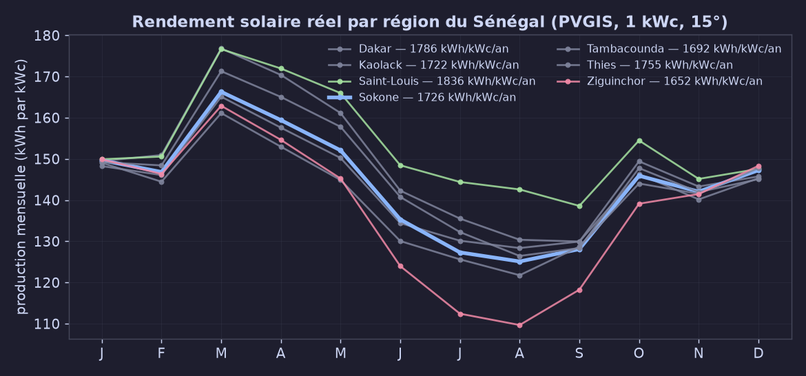
The regional gap is real: Saint-Louis produces 1,836 kWh per kWp and per year, Ziguinchor 1,652, i.e. an 11% gap between the best and the worst site — enough to change a sizing calculation.

Full simulation over 8,760 hours, with a 5 kWh battery (depth of discharge 90%, efficiency 95%):

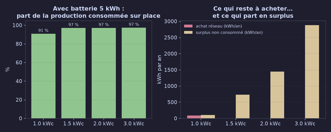
Installed power	No battery: self-consumption	No battery: grid purchase	With 5 kWh battery: self-consumption	With battery: grid purchase	Annual surplus
1.0 kWp	37.6%	860 kWh	90.8%	88 kWh	101 kWh
1.5 kWp	41.3%	809 kWh	97.0%	1 kWh	728 kWh
2.0 kWp	43.5%	779 kWh	97.1%	1 kWh	1,446 kWh
3.0 kWp	46.4%	739 kWh	97.3%	0.5 kWh	2,880 kWh

Three lessons, valid well beyond Senegal:

Without storage, solar works when the house is not consuming. The production peak is at noon, the consumption peak at 8 p.m.
The battery changes everything: self-consumption goes from ~40% to 90–97%.
Oversizing brings nothing to the house: from 1.5 kWp onwards, grid purchase is already almost nil; the extra kilowatts go into surplus. That surplus has a value — solar pumping for irrigation, outdoor lighting, a workshop — but only if it is used.

6.6 How much does it save, in CFA francs

SENELEC tariffs applicable on 1 January 2026 (approved grid, Domestique Petite Puissance — Domestic Small Power — category):

Monthly bracket	Energy price
0 to 150 kWh	82.00 FCFA/kWh
151 to 250 kWh	136.49 FCFA/kWh
More than 250 kWh	159.36 FCFA/kWh

(the 1st bracket fell by 10% on 1 January 2026; a fixed monthly charge depending on the subscribed power and a rural electrification levy of 0.7 FCFA/kWh already included are added to it)

With a consumption of 1,378 kWh/year, the whole consumption stays in the first bracket:

annual consumption to cover: 1,378 kWh × 82 FCFA ≈ 113,000 FCFA per year;
with 1.5 kWp + a 5 kWh battery, grid purchase falls to ~1 kWh/year: the annual saving is therefore of the order of 113,000 FCFA (excluding the fixed charge).

In other words: solar mainly replaces a modest but real bill, and its profitability depends on the price of the installed kit, not on the kWh saved. This is a calculation to be redone with a real quotation — the surplus that is not valued is, for its part, an investment that sleeps.

7. When to use a foundation model (and when to avoid it)

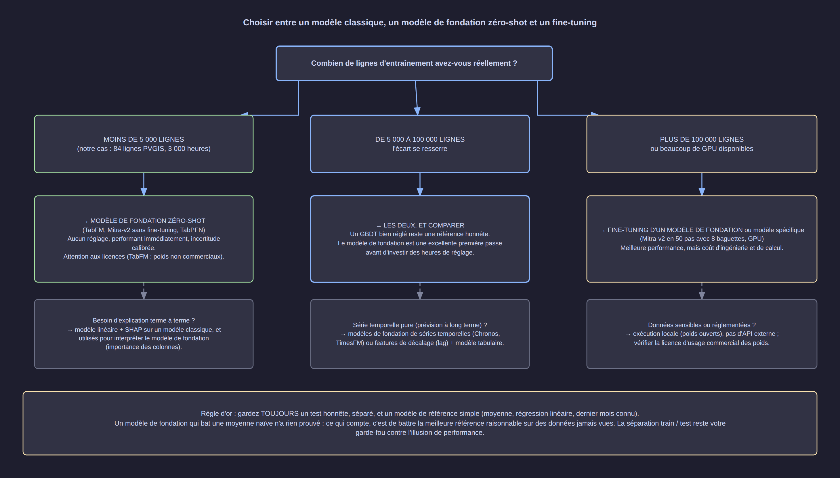
Fewer than a few thousand rows (our case) → a zero-shot foundation model is relevant: effective immediately, uncertainty often better calibrated, zero tuning.
Between a few thousand and a few hundred thousand rows → do both and compare: a well-tuned boosted tree remains a formidable baseline.
Large volumes or production constraints → fine-tuning a foundation model (see the article on Amazon Mitra-v2) or a specific model, trained on your domain.
Pure time series (forecasting the production of the next 30 days) → foundation models dedicated to time series, or lag variables + a tabular model (our experiment B).

8. Limits and pitfalls to know

A foundation model is not proof. It gives a fast first answer that is often good; it does not remove the need for a separate, honest test set.
Context costs memory. These models pass all your training rows at every prediction: memory consumption grows with the number of rows. It is made for small and medium data, not for millions of rows.
Licences. TabFM: non-commercial weights. Recent TabPFN: licence acceptance and API key. Mitra-v2: Apache-2.0 (weights, inference code, fine-tuning code).
Synthetic data is a choice, not a detail. The model learns the regularities of its priors: a very particular domain (exotic industrial sensors, text, images) remains outside its terrain.
A "mean" baseline can mislead. On data as structured as 84 rows of solar production, a deterministic curve already does a large part of the work: the model's merit is to come close to it without tuning, not to work magic.

9. Reproducing the experiment

The scripts of this study follow a simple order:

1. fetch_solar_data.py   → downloads NASA POWER (hourly) and PVGIS (monthly) for 7 regions
2. build_dataset.py      → builds the hourly dataset (8,760 rows), the consumption model,
                           the battery/grid balance and the sizing scenarios
3. run_experiment.py     → experiments A, B, C (naive baselines, classic models, zero-shot TabPFN)
4. export_site_data.py   → publishes the data and results as JSON for the web portal

The data and the interactive charts are published on data-science.pauldiop.com, and the source files of each diagram (.drawio) accompany this article: click on a diagram to open it large, then edit the corresponding .drawio.

10. Key takeaways

A tabular foundation model is pre-trained on millions of synthetic tables: it predicts your data by putting it in the context, with no training and no tuning.
On 84 rows or 1,500 hours, this type of model is directly usable — which leaves time for the part that really matters: formulating the right business question.
For a house in Sokone, most of the gain comes from the production + battery pairing, not from oversizing: 1.5 kWp + 5 kWh are enough to cover a consumption of 3.8 kWh/day at more than 97%.
The real saving is read on the SENELEC bracket (82 FCFA/kWh in 2026 for the first 150 kWh per month): solar replaces a modest bill — to be compared with the installation quotation.

Resources

Model card and code: Google TabFM (GitHub) and weights on Hugging Face
Google Research announcement: Introducing TabFM
Model used in the experiment: TabPFN (Prior Labs)
Solar data: NASA POWER and PVGIS (JRC)
Electricity tariffs: SENELEC tariff grid applicable from 1 January 2026 (CRSE)
Companion article: Amazon Mitra-v2 — Tabular Foundation Models and Fine-Tuning