Supervised Models — a Panorama of Strengths, Limits and Use Cases

Last reviewed: 19 September 2026

Édition française : Les modèles supervisés — panorama, avantages, limites et cas d'usage

XGBoost, linear regression, Random Forest, k-NN, SVM, neural networks: which model should you choose, and why? This article reviews the families of supervised models most widely used in real projects, explaining for each one how it decides, what it brings, what it costs and when it is the right tool. Everything is illustrated, and a real benchmark — 14 models, two tasks, three protocols — puts numbers on the differences using solar production data from Senegal.

Companion article: Unsupervised Learning, Time Series and Anomaly Detection — a Panorama (clustering, dimensionality reduction, anomalies, forecasting). For tabular foundation models — TabFM, Mitra-v2, TabPFN — see the two dedicated articles in the Data-Science folder.

1. The minimum vocabulary

Term	What it means, concretely
Variable (column, feature)	what the model is allowed to look at: irradiation, temperature, month, latitude
Target	what we want to predict: a production level, a probability of failure
Training	adjusting the model's parameters to reduce the error on the training data
Generalisation	performing well on data it has never seen — the only objective that matters
Metric	how the error is measured: MAE, RMSE, R², accuracy, recall, F1…
Test set	the portion of the data set aside and looked at once only, at the end

The number-one beginner's mistake is to confuse the first two rows of the table: a model can be excellent on the training data and poor in production. Everything else in this article follows from that distinction.

2. The compulsory baseline: the dumbest possible model

Before any algorithm, we build a baseline: predicting the mean (regression) or the majority class (classification). In our benchmark, the naive mean gives:

Protocol	Mean error (MAE)	R²
Random split	0.2405 kWh/kWp/day	−0.08
Unknown region held out	0.3661 kWh/kWp/day	−0.17

A negative R² means the baseline does worse than predicting the global mean. That is exactly the point of this row: it gives the scale. A model that improves on it only marginally does not deserve a project; a model that improves on it by 60% (see §7) is telling us something about the phenomenon.

3. The four broad families

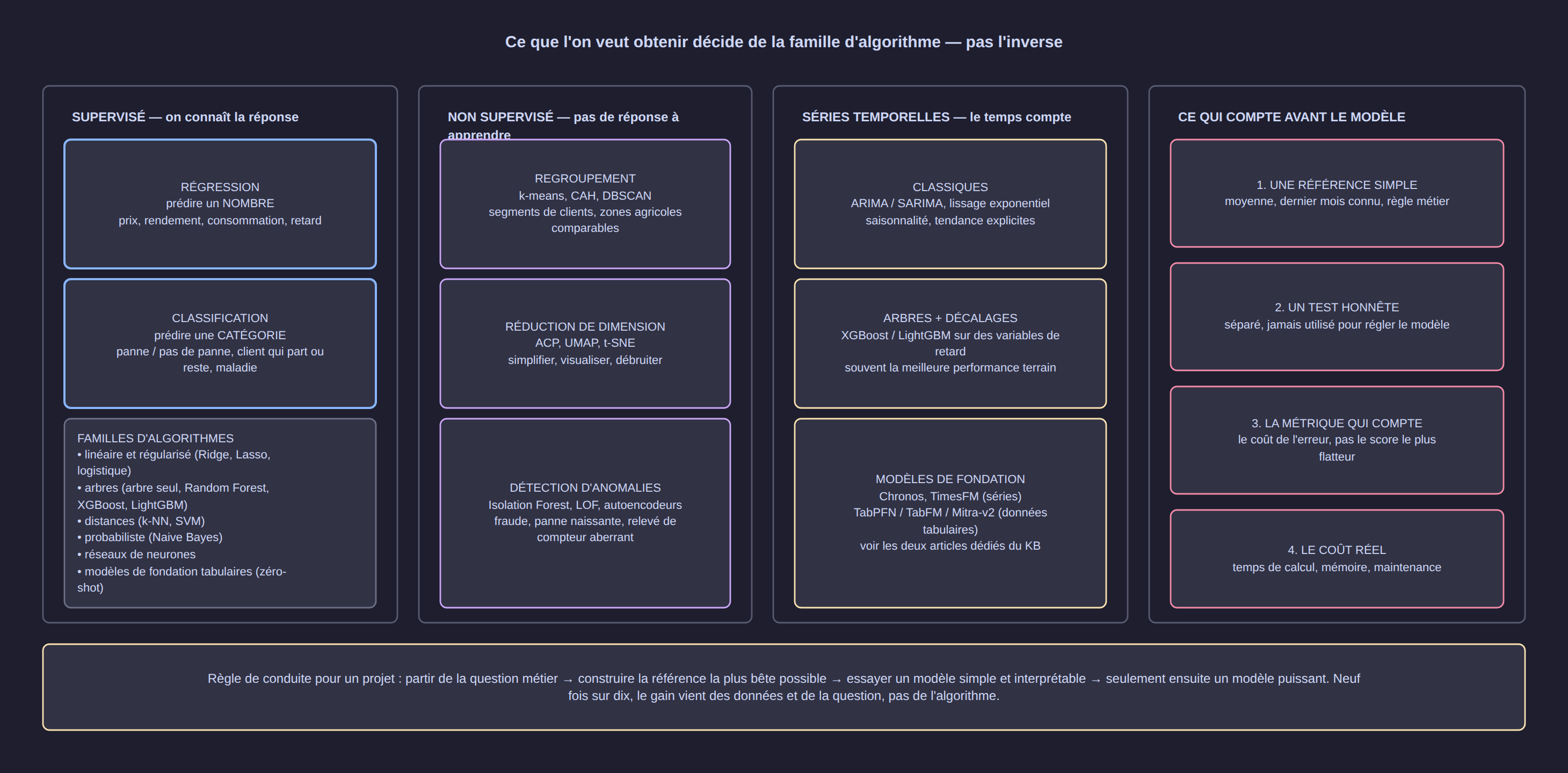
The business question decides the family, never the other way round:

Supervised — the answer is known in the historical data. Two sub-cases: predicting a number (regression) or a category (classification).
Unsupervised — no answer to learn from: we look for a structure (groups, summary, anomaly).
Time series — the variable depends on time, and the order of the rows carries information.
Foundation models — trained once and for all on millions of tasks; they bypass part of the tuning work (dedicated articles).

4. How to read a model's data sheet

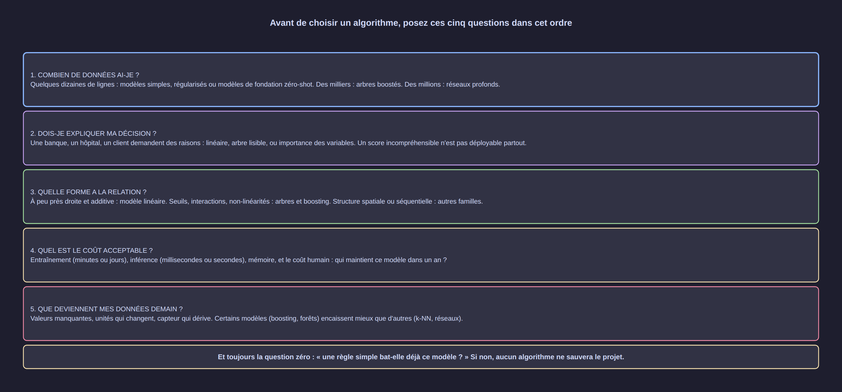
Five questions, in this order: how much data? does the decision have to be explained? what shape does the relationship have? what cost is acceptable? what happens to the data tomorrow? A model is chosen on those five answers, not on a blog ranking.

5. The bias / variance trade-off, or why "more complex" is not "better"

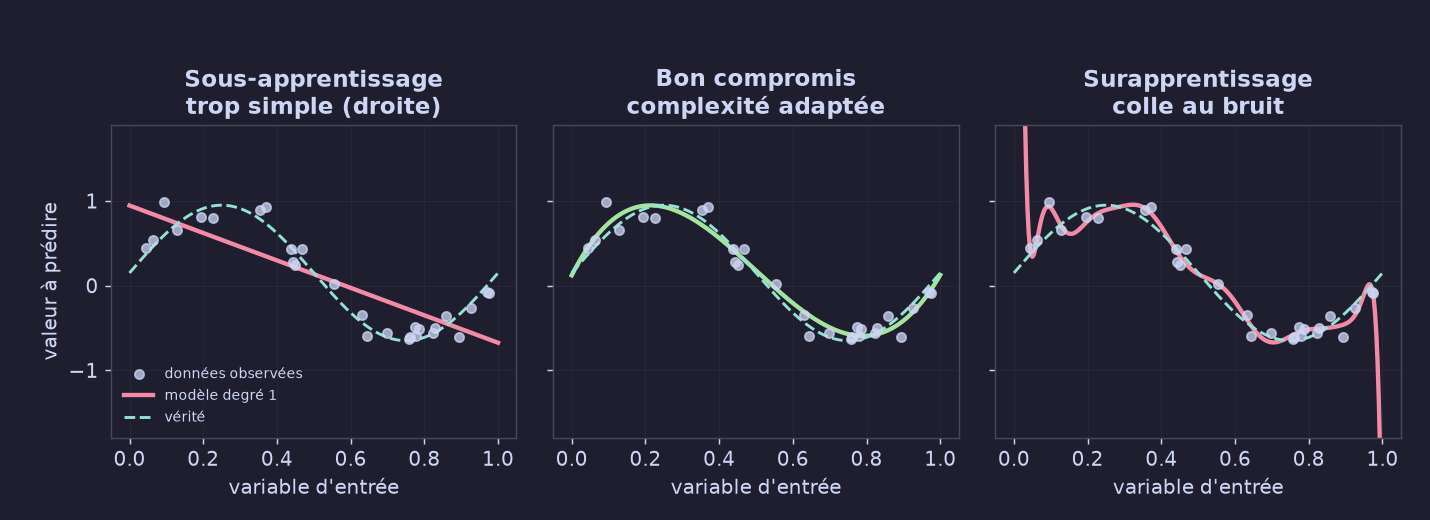
Three models, the same data:

Underfitting (right): the model is too simple to represent reality — high error everywhere.
Good trade-off: the complexity matches the amount of information actually available.
Overfitting: the model hugs the noise. It becomes perfect on the data it has seen and catastrophic elsewhere.

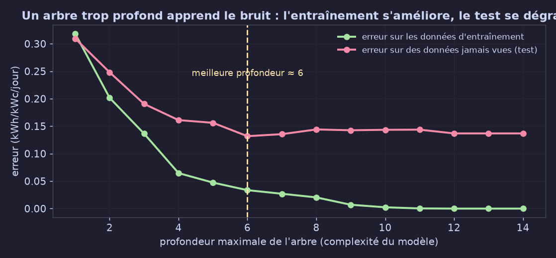
The figure above is computed on our real data: the deeper the tree, the better the training error — and the worse the test error becomes beyond a certain point. This is the central phenomenon of any machine-learning project.

6. The models, one by one

6.1 Linear regression — the line that minimises the gaps

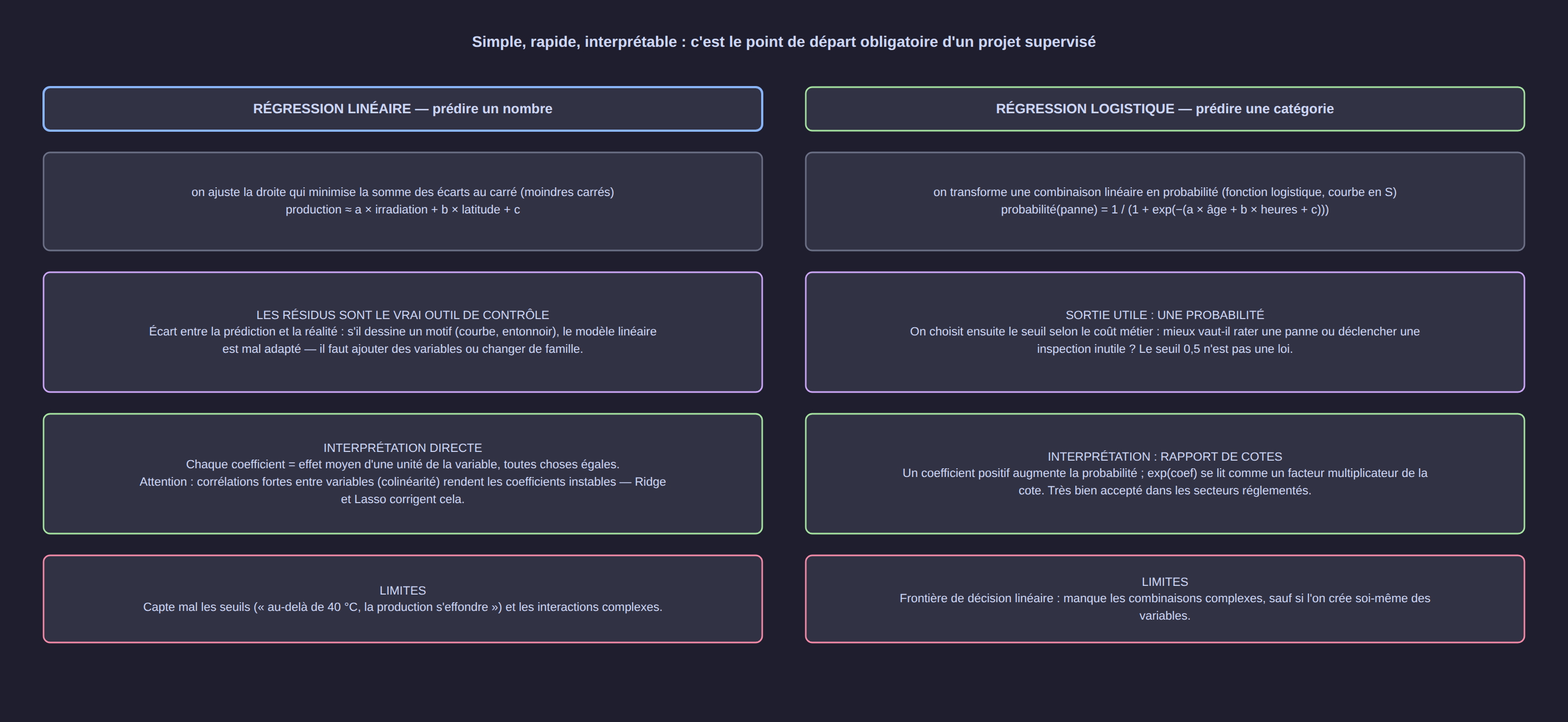
The idea in one sentence: the target is a linear combination of the variables (production ≈ a × irradiation + b × latitude + c).
How it decides: it picks the coefficients that minimise the sum of squared gaps (least-squares method). The residuals (gaps between the prediction and reality) are the checking tool: if they draw a pattern, the model is a poor fit.
Strengths: instantaneous (milliseconds), interpretable (one coefficient = one average effect), works with very few rows, extremely well understood in regulated industries.
Limits: does not capture thresholds or complex interactions; sensitive to outliers; unstable if two variables are highly correlated.
Typical use cases: price estimation, effect of a technical parameter, a project's first model, elasticity calculation, baseline model to beat.
In our benchmark: MAE 0.1039 and R² 0.83 with… 67 training rows. A well-used straight line is already a serious model.

from sklearn.linear_model import LinearRegression
m = LinearRegression().fit(X_train, y_train)
print(dict(zip(features, m.coef_.round(3))), m.intercept_)   # readable straight away

6.2 Ridge, Lasso, Elastic Net — the same, better kept in check

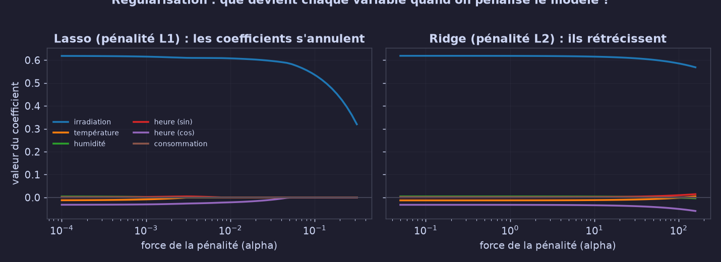
The idea: adding a penalty to stop the coefficients from becoming huge or from cancelling each other out when the variables are correlated.
Ridge (L2) shrinks all the coefficients; Lasso (L1) sets some of them exactly to zero — so it selects variables; Elastic Net mixes the two.
Strengths: more stable than OLS, more resistant to noise, Lasso produces a shorter model and therefore a more explainable one.
Limits: the variables must be standardised (otherwise the penalty bites differently depending on the units); the strength of the penalty is chosen by cross-validation.
Use cases: many correlated variables (redundant sensors, multiple weather readings), need for a short and defensible model.
In our benchmark: Lasso does slightly better than OLS (MAE 0.1035 versus 0.1039), and clearly better when an entire region is unknown (0.1373 versus 0.1412).

6.3 Logistic regression — a probability, not a label

The idea: turning a linear combination into a probability with an S-shaped curve.
How it decides: a threshold is chosen afterwards (and it does not have to be 0.5) according to the real cost of the errors: does missing a failure cost more than a needless inspection?
Strengths: fast, calibrated, interpretable (odds ratios), excellent even with little data; this is the standard in credit risk, medicine and marketing.
Limits: linear decision boundary; imbalanced classes require an explicit adjustment.
In our benchmark: 99.4% accuracy in 7 milliseconds of training — and tens of thousands of times faster at inference than the foundation model that reaches 100%.

6.4 k-nearest neighbours (k-NN) — "tell me who your neighbours are"

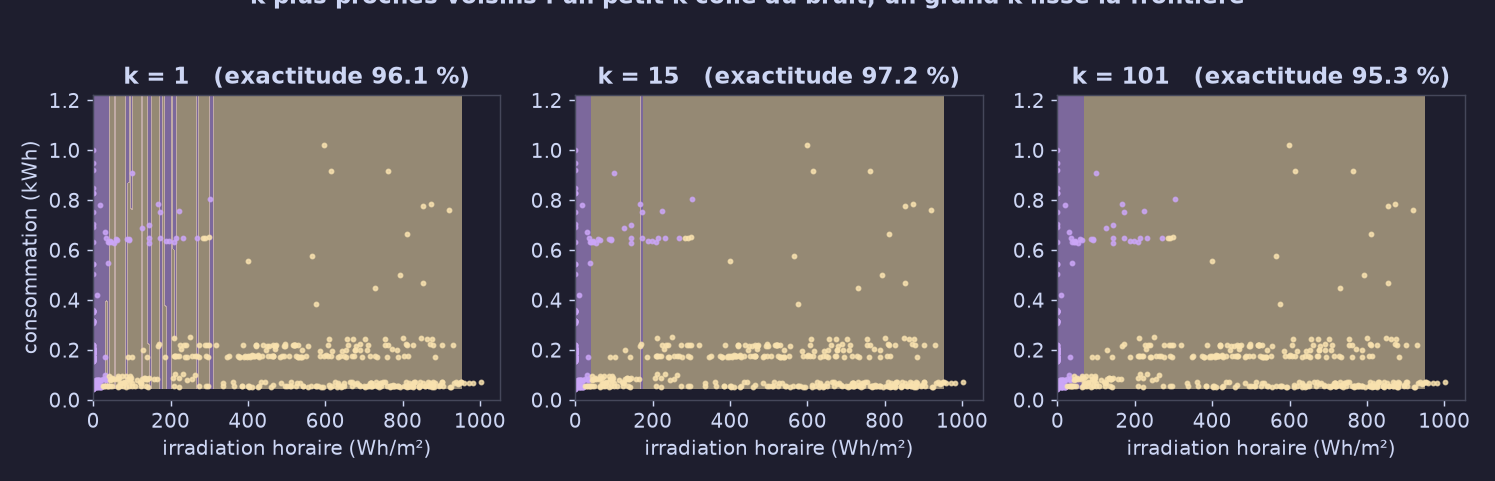
The idea: to predict a point, look at its k nearest neighbours and vote (or average). No training: the whole cost is at prediction time.
The setting that matters: k. Too small, the model follows the noise; too large, it smooths everything out. The figure above, computed on our real data, shows the three regimes.
Strengths: instantly understandable concept, no assumption about the shape of the relationship, trivial to implement.
Limits: suffers from the curse of dimensionality (with 20 variables, everyone is "far away"), requires scaling, sensitive to useless columns, slow in production.
Use cases: simple recommendation systems, similarity checks, geographic proximity labelling.
In our benchmark: the worst of the classical models in regression (R² 0.56), average in classification (97.8%) — one of the few cases where a simple method pays poorly.

6.5 Decision tree — a sequence of readable questions

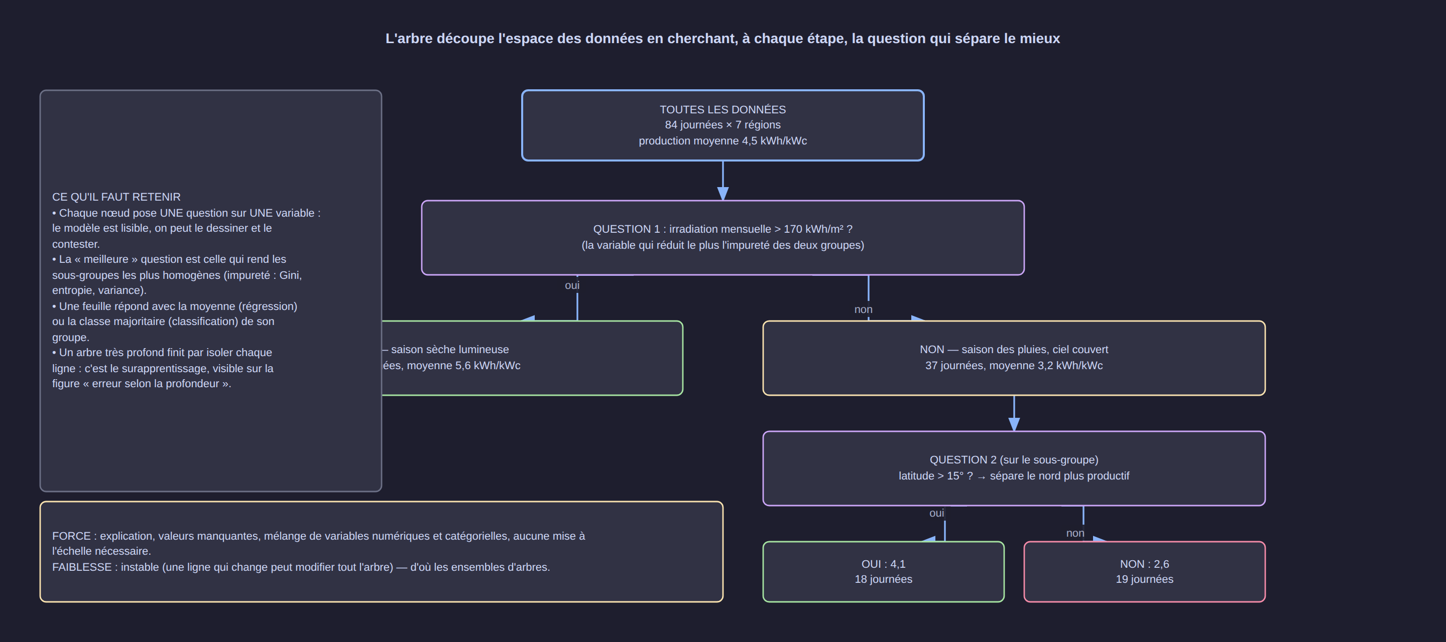
The idea: at each node, one question about one variable, chosen to split the data as well as possible; a leaf answers with the mean or the majority class of the group.
Strengths: explanation in plain language, missing values tolerated, a mix of numerical and categorical variables, no scaling, interactions detected automatically.
Limits: very unstable (changing one row can change the whole tree) and it overfits quickly — hence the "error versus depth" figure above, and hence ensembles of trees.
Use cases: decision rules to be validated by experts, a simple risk score, a basis for discussion with the business side.
In our benchmark: a single tree of depth 4 is enough to reach 99.8% in classification — an excellent readability/performance ratio.

6.6 Random Forest and Extra Trees — a vote of several trees

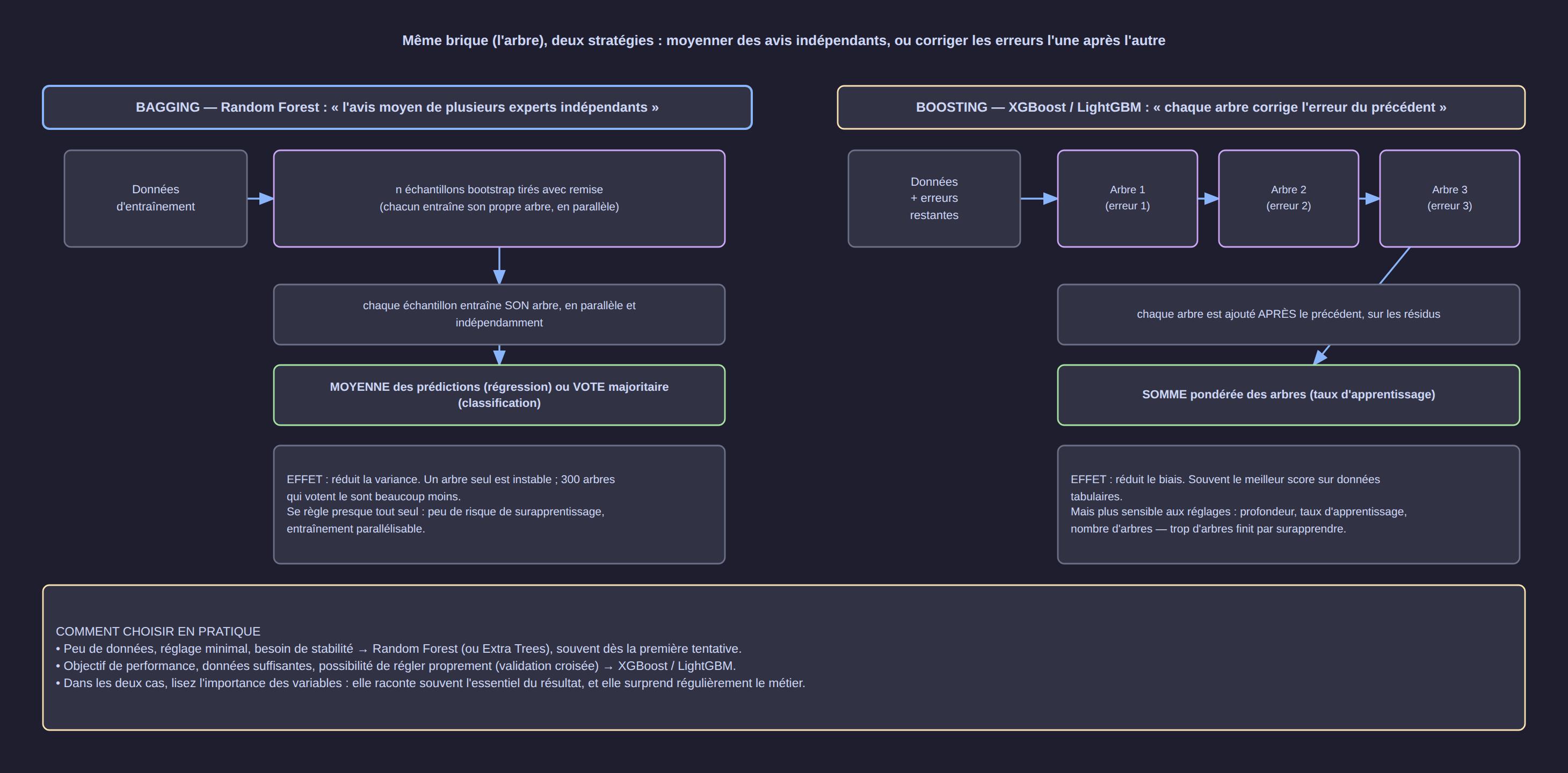
The idea (bagging): training hundreds of trees on samples drawn with replacement and on subsets of variables, then averaging their predictions. Each tree is wrong in a different way; the errors partly cancel out in the average.
Extra Trees: the same principle, but the split thresholds are drawn at random — faster, often just as accurate, a little more "smoothed".
A single parameter to tune seriously: the number of trees (300 is plenty in practice).
Strengths: very robust, little tuning, parallelisable, provides feature importance, copes with outliers and missing values.
Limits: less accurate than boosting on many tabular data sets; a bulky model in memory; can be biased on highly imbalanced classes.
Use cases: the first "serious" model of a tabular project, estimation of feature importance, data with many noisy columns.
In our benchmark: MAE 0.0878 (R² 0.88) under random split; 0.1023 (R² 0.90) on an unknown region — the best "classical" family.

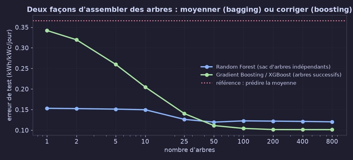
6.7 Gradient boosting: XGBoost, LightGBM, CatBoost

The idea (boosting): building trees one after another, each one learning to correct the remaining errors of the previous ones, then summing the whole thing with a small step (learning rate).
Why it works so well on tabular data: each tree focuses on the difficult examples, which greatly reduces bias — and it often beats neural networks on medium-sized tabular data.
The three variants: XGBoost (the most established), LightGBM (the fastest on large volumes), CatBoost (the simplest with categorical variables).
Settings that really matter: number of trees, learning rate (0.03–0.1), depth or number of leaves, and subsampling. Too many trees without control = overfitting.
Limits: a relative black box (mitigated by SHAP), more tuning than a Random Forest, can overfit on small noisy data sets.
Use cases: competitions, scoring, demand forecasting, fraud detection, any project where you are chasing the last points of performance.
In our benchmark: XGBoost better than Random Forest under random split (0.0844) but worse when an entire region is unknown (0.1107 versus 0.1023): boosting exploits the regularities it has seen well, extrapolation a little less well.

6.8 SVM (support vector machines)

The idea: finding the boundary that separates the classes by maximising the margin, with a kernel to handle curved boundaries.
Strengths: effective on medium-sized data with many variables (text, spectra, simple images), a solid theoretical basis, little overfitting with a good margin.
Limits: scales poorly (quadratic complexity in the number of rows), delicate tuning (C, gamma), no direct interpretation, no native probabilities.
Use cases: classification of short texts, signature detection, small high-dimensional data sets.
In our benchmark: 98.0% in classification; on the other hand R² 0.48 when a region is unknown — fragile outside its training domain.

6.9 Naive Bayes

The idea: applying Bayes' theorem while assuming (wrongly but effectively) that the variables are independent.
Strengths: very fast, works with little data, excellent for text (spam filters, document sorting), provides probabilities.
Limits: the independence assumption is rarely true; the probabilities are poorly calibrated.
In our benchmark: 96.2% accuracy — the lowest of the non-trivial models, but with the shortest training time (1 ms).

6.10 Neural networks (multilayer perceptron)

The idea: stacking layers of non-linear transformations to learn complex relationships.
Strengths: excellent on images, text and sound; captures very complex interactions; improves with data and compute.
Limits on tabular data: requires a lot of data and a lot of tuning, gives no direct explanation, and extrapolates very badly outside the domain seen during training.
Our benchmark's counter-example is spectacular: under random split the MLP reaches R² 0.34; when an entire region is unknown, it collapses to R² −18.3 (MAE 1.11 versus 0.14 for a linear regression). In other words: with 84 rows, a neural network has no place — and the benchmark proves it with the numbers in hand.
Use cases: as soon as there is a lot of unstructured data; almost never as a first choice on a table of 100 to 10,000 rows.

6.11 Tabular foundation models (for the record)

Pre-trained on millions of synthetic tables, they predict through in-context learning, with no training or tuning. In our benchmark, zero-shot TabPFN v2 is the best of the 14 models in regression (MAE 0.0362, R² 0.98) as well as in regional extrapolation (MAE 0.0858) — but it is slow at inference on CPU (833 s for 495 rows) and its weights have to be checked depending on the vendor (licence, API key). Full details in the two dedicated articles.

7. The benchmark: 14 models, two tasks, three protocols

Everything is reproducible (scripts provided) and computed on the data from the Badoudou solar case: real photovoltaic production (PVGIS, 7 regions, 12 months) and the modelled consumption of a household.

7.1 Regression — predicting daily production

Protocol 1: random split (67 training rows, 17 test rows).

Model	MAE	R²	Training
Naive mean (baseline)	0.2405	−0.08	—
TabPFN v2 (zero-shot)	0.0362	0.98	0.41 s
XGBoost	0.0844	0.85	0.12 s
Extra Trees	0.0857	0.90	0.19 s
Random Forest	0.0878	0.88	0.28 s
Lasso	0.1035	0.84	0.004 s
Linear regression	0.1039	0.83	0.009 s
Decision tree (depth 4)	0.1053	0.79	0.004 s
Ridge	0.1059	0.83	0.007 s
HistGradientBoosting	0.1139	0.84	0.05 s
SVM (RBF kernel)	0.1173	0.80	0.003 s
LightGBM	0.1259	0.76	0.03 s
k-nearest neighbours (k=5)	0.1647	0.56	0.005 s
Neural network (MLP)	0.2006	0.34	0.14 s

Protocol 2: an entire region held out (the hardest test; average over 7 regions).

Model	Mean MAE	Worst region	R²
TabPFN v2 (zero-shot)	0.0858	0.190	0.93
Extra Trees	0.0962	—	0.92
Random Forest	0.1023	0.183	0.90
XGBoost	0.1107	—	0.88
Decision tree	0.1272	—	0.84
Lasso	0.1373	—	0.82
Linear regression	0.1412	0.234	0.81
k-nearest neighbours	0.1593	—	0.79
HistGradientBoosting	0.1558	—	0.81
LightGBM	0.1650	—	0.79
SVM (RBF kernel)	0.2223	—	0.48
Naive mean	0.3661	—	−0.17
Neural network (MLP)	1.1098	—	−18.3

7.2 Classification — surplus or deficit, hour by hour

1,005 training hours, 495 test hours.

Model	Accuracy	F1	Training	Prediction (500 rows)
Majority class (baseline)	55.6%	0.000	—	—
LightGBM	100.0%	1.000	0.07 s	0.005 s
Decision tree (depth 4)	99.80%	0.998	0.002 s	< 0.001 s
HistGradientBoosting	99.80%	0.998	0.14 s	0.008 s
XGBoost	99.80%	0.998	0.06 s	0.003 s
Random Forest	99.60%	0.996	0.39 s	0.120 s
Extra Trees	99.39%	0.993	0.34 s	0.131 s
Logistic regression	99.39%	0.993	0.007 s	0.003 s
Neural network (MLP)	99.19%	0.991	0.53 s	0.003 s
SVM (RBF kernel)	97.98%	0.977	0.03 s	0.008 s
k-nearest neighbours	97.78%	0.975	0.002 s	0.011 s
Naive Bayes	96.16%	0.956	0.001 s	0.001 s
TabPFN v2 (zero-shot)	100.0%	1.000	0.19 s	833 s

7.3 How to read this benchmark (five lessons)

The baseline first. 55.6% in classification and a negative R² in regression: that is what has to be beaten. Every serious model beats it by a wide margin.
The best model depends on the protocol. XGBoost leads Random Forest under random split, the opposite when an entire region is unknown. A ranking is never absolute.
Little data changes everything. With 84 rows, neural networks and SVMs fall away; regularised models and forests hold up; the zero-shot foundation model dominates.
Cost matters. The most accurate model can be tens of thousands of times slower at inference. On an almost deterministic task (everyone is between 99% and 100%), logistic regression is the rational choice.
A simple, well-understood model often beats a complex, badly tuned one — and it can be defended in a meeting, which is not a detail.

8. Selection guide

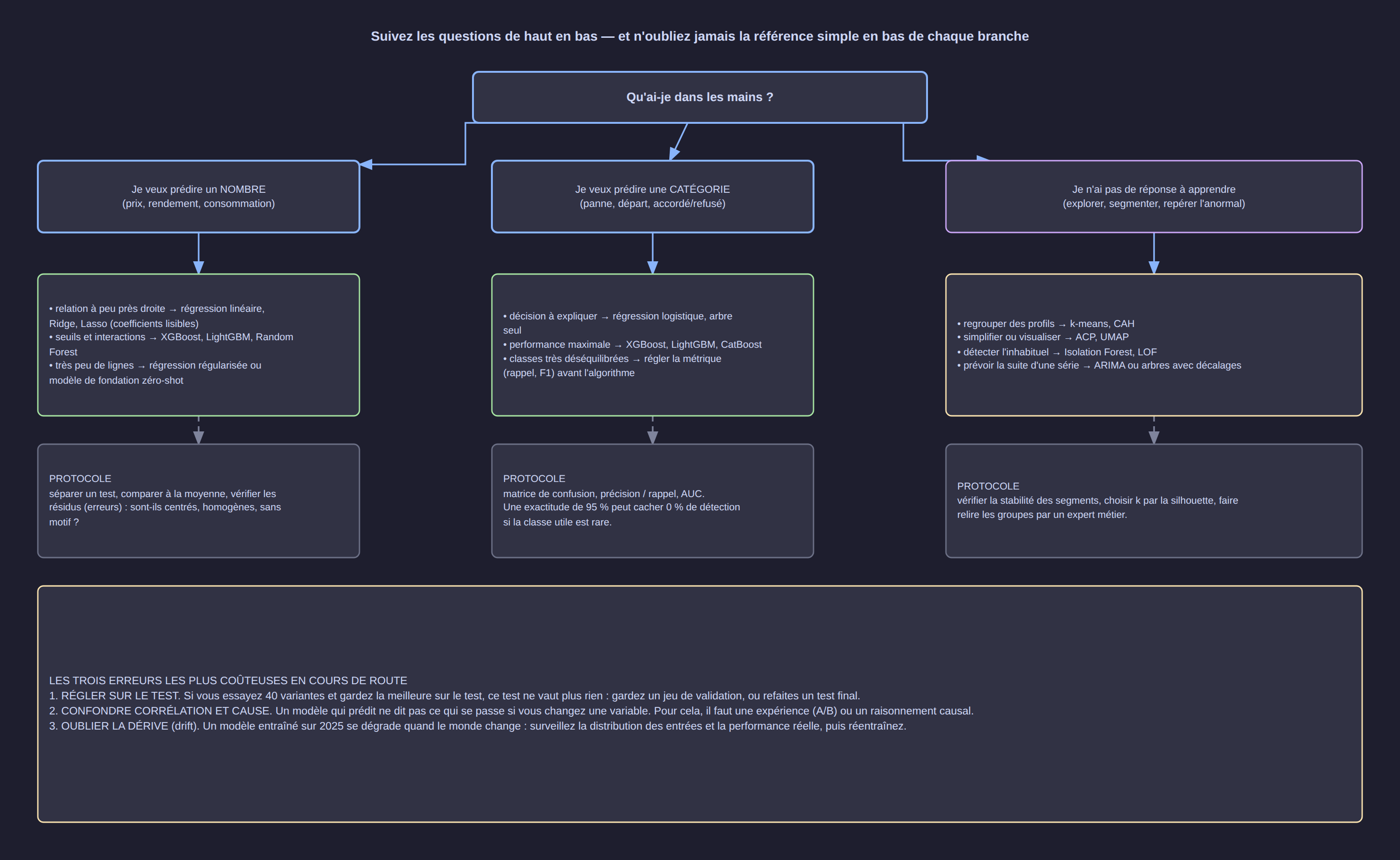
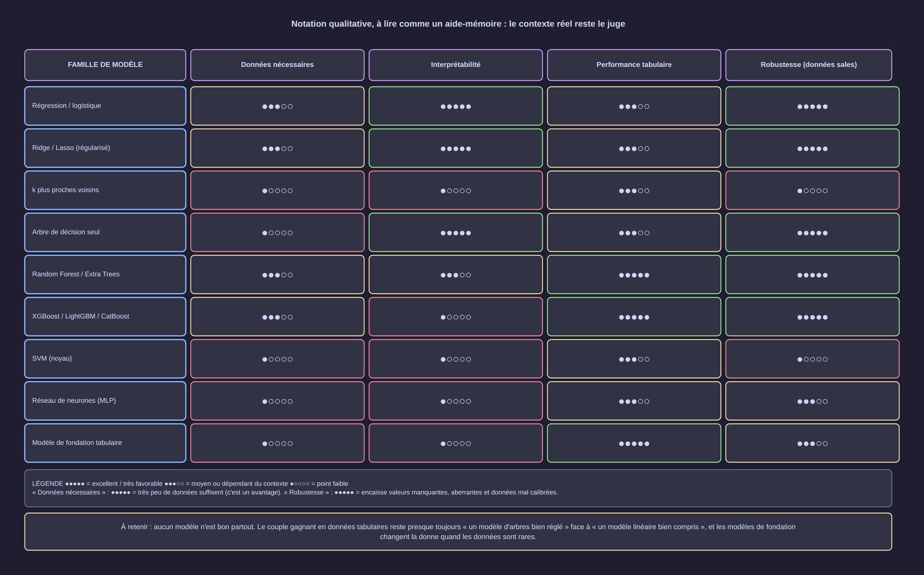
The useful shortcut for a typical tabular project:

Always first: a baseline (mean / majority class) and, if the variables are few, a linear or logistic regression — for interpretation and as a point of comparison.
Then: a Random Forest (little tuning, robust) or XGBoost/LightGBM (performance) — and compare honestly.
Very scarce data (< 1,000 rows): a zero-shot tabular foundation model changes the picture; regularised regression remains an excellent base.
Many columns, few rows: Lasso/Ridge or kernel models, plus dimensionality reduction (see the companion article).
A lot of unstructured data: deep networks — that is their home ground.

9. The five mistakes that cost you dearly

Tuning the hyperparameters on the test set. After 40 attempts, the "best" score is a lucky accident. Use a separate validation set, then a single final test.
Forgetting the baseline. Without it, there is no way to know whether the model adds anything.
Confusing prediction with causation. A model predicts; it does not say what happens if you change a variable. For that: a controlled experiment or causal reasoning.
Ignoring class imbalance. 95% accuracy can mean "detects nothing" when the useful class accounts for 5% of cases: look at recall and F1.
Monitoring nothing in production. Data drifts (prices, hardware, behaviour). Without monitoring the distribution of the inputs and the real performance, the model degrades silently.

10. A seven-step working method

Formulate the decision the model is meant to inform (not "predict X", but "decide what, when, with what acceptable error").
Build the table: one row = one case, one column = one piece of information available on the decision date.
Set the simple baseline and the metric that matches the real cost of the error.
Split the data (train / validation / test), respecting time when the data is temporal.
Try two or three families, not fifteen: an interpretable linear model, a tree ensemble, possibly a foundation model.
Read the errors: where does the model go wrong? Is there a pattern (a region, a season, a type of customer)? That is where the next gain lies, not in the choice of algorithm.
Deploy, measure, retrain: version the model and the data, monitor drift, plan the date of the next retraining.

11. Key takeaways

The families that cover most real work: regularised linear models, single trees, tree ensembles (bagging), boosting (XGBoost/LightGBM/CatBoost), distance-based (k-NN, SVM), probabilistic (Naive Bayes), neural networks — and now foundation models.
On small or medium-sized tabular data, tree ensembles remain the reference, linear models provide the explanation, and foundation models shine when the data is scarce.
The gain rarely comes from the algorithm: it comes from the question asked, from the quality of the table and from the honesty of the test protocol.
A model is chosen on four simultaneous criteria: performance, explainability, cost, robustness — exactly the columns of the matrix in §8.

Resources

Benchmarks and scripts: the data and the figures are published on the data-science.pauldiop.com portal; the code for the experiments accompanies the Badoudou solar project.
Reference documentation: scikit-learn — supervised learning guide, XGBoost, LightGBM, CatBoost
Interpretation: SHAP for explaining tree models
Related articles: Google TabFM — Tabular Foundation Models (zero-shot forecasting) and Amazon Mitra-v2 — Tabular Foundation Models and Fine-Tuning; companion article: Unsupervised Learning, Time Series and Anomaly Detection — a Panorama